Physical Mediums & Transceivers
Copper vs Optical — Which to Pick?
Both copper and optical cables offer differentiating advantages and disadvantages over the other, and picking one at first might seem simple — but like everything in reality, it gets complex as the technological framework and architectures get more complex, and with the added economical impacts each has.
The best way to make a correct decision is by understanding each medium’s advantages and disadvantages and comparing them to the situation at hand.
By examining the situation more broadly and applying those advantages and disadvantages at strategic points, we can determine the best solution. Worthy to note: there is no “bad solution.” It dials down to “less ideal” vs “more preferable,” as each medium also comes with disadvantages worth noting.
| Property | Copper | Optical |
|---|---|---|
| Cost | Overall cheaper full ownership | More expensive; requires pricier equipment, SFPs, Testing Equipment etc. |
| Distance | Shorter runs | Further lengths |
| Bandwidth | Competitive at short reach; practical ceilings fall sooner as distance grows | Higher practical speeds over longer distances |
| Ease of use | Widespread and easy to get | More specialized tooling and handling |
| Availability | Common and easy to source | Widely available; faster-evolving ecosystem |
| Durability | Less Fragile, more rugged and tolerant to rough handling | More fragile (bend radius and dirt); more malleable in racks |
| Interference | More prone to EM interference | No EM interference |
| Rack organization | More rigid; at scale, more annoying to organize | Easier to organize in racks |
| Link utilization | One signal per link | CWDM & DWDM allow more per-link utilization (many wavelengths on one link) |
| Heat | Depends on the interface: passive copper runs cool, while active 10GBASE-T PHYs can be power-hungry | Pluggable optics add module heat; higher-rate and coherent optics can add substantially more |
| Repair & Installation | field-terminable with basic tools, no splicing | Harder (splicing vs copper) |
Please note that DACs and AOCs were removed from the equation, but they do follow a similar trend. Generally speaking, each also has its own advantages and disadvantages and might be beneficial in some use cases and not in others.
Knowing these pieces of information makes a decision far easier to make. Need a long-haul connection? Optical. Need a bunch of IP cameras that sit outside? Copper. What about a lot of density in datacenters? Here’s where it gets trickier. Whilst saying optical might be an easy decision, note the disadvantages of optical — heat, which becomes very prevalent today, increased cost, and so on — meaning it is no longer as easy of a decision, and requires further digging into the requirements. What’s the cooling solution in the datacenter to accommodate optical vs what’s the expected bandwidth and future growth? Perhaps DACs offer a better solution compared to optical in such a scenario.
It comes down to, there is no right or wrong — but there are trade-offs and considerations. so, It dependsTM
Single-mode vs Multi-mode untangled
In optical cabling, there are two main “modes” of operation. Each is not an advancement over the other, but rather a solution for a specific problem, that evolved over time into a different market of the same branch of optics.
Almost all cables regardless of their mode are built similarly: a core comprised of silica/glass, surrounded by a cladding for protection. Some might offer better cladding compared to others, or specific materials used in the core, but the general idea persists.
Before examining the types, let’s go through some worthy-to-know attributes and their meaning to fully comprehend the cable’s characteristics.
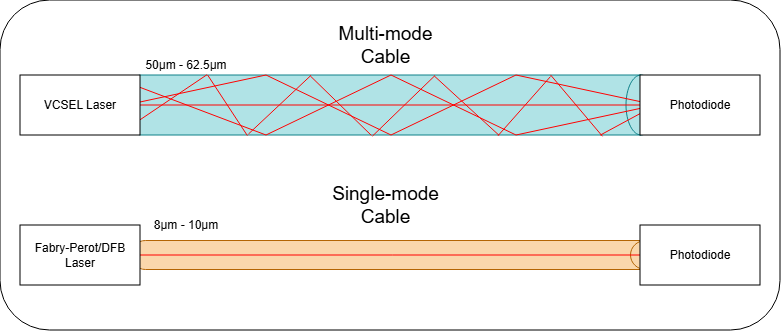
- Smearing — Smearing is the result of a principle in optical fibers called modal dispersion and is only relevant for multi-mode cables. Light is sent in at different angles and travels along multiple paths (modes) of differing lengths, so parts of the same pulse arrive at slightly different times. This results in a distorted or sometimes unreadable pulse (data loss).
Single-mode
Single-mode cables are characterized by a smaller core (8–10μm diameter). This smaller core only permits a single path of light to propagate, so there is no multi-path spreading to begin with.
Multi-mode
Multi-mode cables are characterized by a larger core (50μm to 62.5μm). The larger core introduces reflections of the light from the laser in the transceiver, which can lead to lightwaves taking different paths, and as a result reaching the other side at different times, which adds smearing.
Why use each?
Single-mode is created with the goal of distance and bandwidth. This means you cannot afford a larger core that results in the aforementioned drawbacks, and it also means you need better hardware to achieve such distances and speeds. The transceivers used in single-mode applications are inherently more expensive by using better light sources with higher precision (Fabry-Perot/DFB).
Multi-mode is a result of cost-saving. A larger core allows for more head-room in precision, meaning the transceivers themselves are far cheaper to manufacture, and so is the laser itself (usually VCSELs). That’s also the main reason why they’re only meant for short range: the bigger core introduces more smearing, and the lower cost adds less manufacturing accuracy that can also contribute.
Transceiver form-factors
Throughout history, different transceiver types were introduced. At first glance the main driver was increased bandwidth — but while true, that hides the more niche needs that evolved over time, such as distance, medium conversion, wavelength specifics, tunable optics, breakouts, and even environmental hardening.
This portion focuses primarily on transceivers for optical connections, as opposed to DACs.
The two levers
Before the list, one framing that makes every form factor self-describing. Total throughput is the product of two independent levers:
- Lane count — encoded in the prefix. SFP = 1 lane, QSFP (Quad) = 4 lanes, OSFP (Octal) = 8 lanes. “DD” (Double Density) doubles the base: SFP-DD = 2 lanes, QSFP-DD = 8 lanes.
- Per-lane rate — encoded in the suffix number. The “28” in SFP28/QSFP28 refers to the ~28 Gbps lane rate (25G of data plus encoding overhead), “56” ≈ 50G/lane, “112” ≈ 100G/lane.
So QSFP28 reads as 4 lanes × ~25G = 100G, and OSFP (8 lanes) at 100G/lane = 800G. A future 200G-per-lane part slots straight into this framework without rethinking it — which is why the principle ages better than any fixed speed number.
SFP family (1 lane)
| Form factor | Year (approx.) | Lanes | Per-lane | Total | Notes |
|---|---|---|---|---|---|
| SFP | 2001 | 1 | 1G | 1G | Replaced GBIC. Variants: MII (100M), SGMII (1G) |
| SFP+ | 2006 | 1 | 10G | 10G | Still a dominant format today |
| SFP28 | 2014 | 1 | 25G | 25G | Same footprint as SFP+; IEEE 802.3by |
| SFP56 | ~2019 | 1 | 50G | 50G | PAM4 signalling |
| SFP-DD | 2019 | 2 | 50G | 100G | Double-density; also supports 200G via PAM4 |
QSFP family (4 lanes, unless doubled)
| Form factor | Year (approx.) | Lanes | Per-lane | Total | Notes |
|---|---|---|---|---|---|
| QSFP (original) | ~2006 | 4 | 1G | 4G | Original spec (4×1G); rarely referenced today |
| QSFP+ | 2012 | 4 | 10G | 40G | Dominant 40G format; MPO-12 or LC duplex |
| QSFP28 | 2014 | 4 | 25G | 100G | Also 2×50G variant, but 4×25G→100G dominates |
| QSFP56 | 2019 | 4 | 50G | 200G | PAM4 |
| QSFP112 | 2021 | 4 | 100G | 400G | Backwards compatible with QSFP56/QSFP28 |
| QSFP-DD | — | 8 | 50G | 400G | Double-density (8 lanes); PAM4 |
| QSFP-DD800 | — | 8 | 100G | 800G | 800G evolution; competes with OSFP |
OSFP family (8 lanes)
| Form factor | Year (approx.) | Lanes | Per-lane | Total | Notes |
|---|---|---|---|---|---|
| OSFP (400G) | products ~2019 | 8 | 50G | 400G | First generation; slightly larger than QSFP for more power/heat headroom |
| OSFP (800G) | products ~2022 | 8 | 100G | 800G | 800G evolution; QSFP backward-compat via adapter where the host supports it |
| OSFP-XD | current frontier (as of 2026) | 16 | 100G | 1.6T | Separate extended-density, 16-lane form factor |
Backwards compatibility
Higher-tier ports generally accept older modules, but only in one direction: a newer port can auto-negotiate down to run an older module (e.g. a QSFP+ module works in a QSFP28 port at 40G), but an older port cannot drive a newer module — a QSFP28 module will not link up in a QSFP+ port, because the older port’s ASIC can’t handle the higher per-lane electrical rate. The same one-way rule applies to the SFP line and to QSFP-DD’s ability to downgrade 8 lanes to 4/2/1.
NRZ vs PAM4
NRZ and PAM4 are modulation methods. The easiest way to understand the role they play in the grand scheme of things is by walking through how they work.
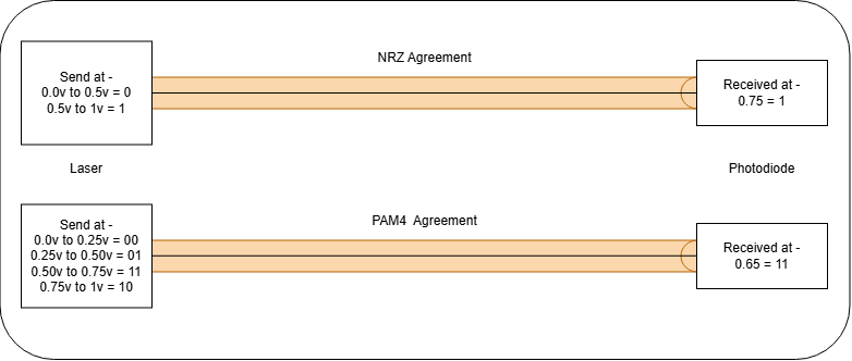
Imagine a laser and a photodiode — essentially the two ends of a cable and a transceiver. The laser is the TX and the photodiode is the RX. The laser is responsible for sending a pulse of light, and the photodiode is responsible for translating that light into voltage.
The following example is illustrative — the numbers might be off.
With NRZ, there is a single threshold that matters. Let’s assume “bright = 1 vs dim = 0.” If I send a very bright pulse (even with attenuation, the loss of power due to distance), it would still be brighter than a dim pulse. The photodiode on the other end would receive that and translate it into 0.9 volt. That means that specific pulse was a 1. The reason it was a 1 is because NRZ’s threshold is at the middle (0.5 volt), so anything above that is a 1. The same goes for sending a dim pulse: when it is received on the photodiode, let’s assume it is received and converted at 0.2 volt — this would mean it’s a 0 according to the NRZ threshold. This is how you send 1 bit per pulse of light.
PAM4, on the other hand, has 4 levels (separated by 3 thresholds). Let’s assume for example: “dim = 0.0 to 0.25 volt, less dim = 0.25 to 0.50 volt, less bright = 0.50 to 0.75 volt, and bright = 0.75 to 1 volt.” The two sides have a mutual agreement on the modulation, and the laser has the responsibility of sending pulses according to the levels set above. They translate to dim = 00, less dim = 01, less bright = 11, bright = 10 — the result is the ability to send 2 bits for each pulse.
Assume the laser intends to send a single pulse that represents 01. It knows to send it with a brightness that translates to “less dim,” or 0.25 to 0.50 volt, when it reaches the other side. The brightness sent by the laser needs to be received by the photodiode at the right level to translate it from light to volt at 0.25 to 0.50 volt.
Whilst a little convoluted, this is how you can increase the total bandwidth (by increasing the total bits sent) on the same cable and hardware. This requires more precision on both the photodiode and the laser — and here’s why: because four levels are packed into the same 0–1 volt range, the gaps between them (and the margin to each threshold) are roughly a third of what they were with NRZ. That means the same amount of noise that was harmless with NRZ can now push a reading across a threshold and into the wrong level, so PAM4 has a higher raw error rate and leans on stronger forward error correction (FEC) to recover. In short, PAM4 buys more bits per pulse, and the tighter margins are the price.
A general rule of thumb is that the optical per-lane rate loosely indicates the modulation: 25G per lane and below is usually NRZ, while 50G per lane and above is usually PAM4 — the industry jumped straight from one to the other, so nothing sits between.
Wavelengths and Bands
As Wikipedia states, “a wave is a propagating dynamic disturbance (change from equilibrium) of one or more quantities.” Very loosely (and loosely matters here), a wave can be viewed as a cycle that moves through space, and as it moves, it interacts with and is affected by its surroundings. An easy way to picture it is throwing a stone into a lake: in the splash area, waves are generated from the energy of the impact of the rock hitting the surface of the water, and those waves then propagate outward. The impact generates energy, the energy needs somewhere to go, and the waves are what moves it.
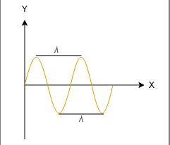
A wavelength is measured between two adjacent points in the same phase on the wave. The lambda (λ) marks the wavelength; in such an example, it doesn't matter which λ is picked — since the two points are in the same phase, the wavelength would always be the same.
Refraction and dispersion
Before moving further, it’s worth mentioning two additional important physics phenomena — refraction and dispersion — and what the refractive index is.
Refractive index is a unitless number that measures how much a material slows down light compared to a vacuum. For example, air has a refractive index (denoted as N) of 1.0003 (almost no slowdown, hence no redirection), and water has N = 1.33 — that's why you can see the redirection of light when placing an item within water.
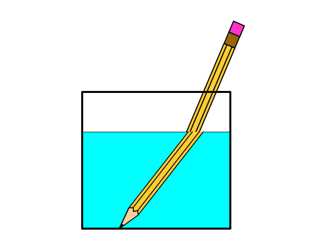
Refraction is the result of a light wave moving from one medium to another (air to water, for example). The redirection is caused by the change of speed that occurs when the light enters from either a higher or lower refractive index into the other medium; higher or lower indicates the direction.
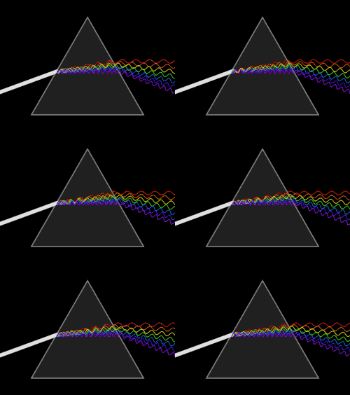
The prism illustrates angular dispersion: different wavelengths refract at different angles. In fiber communications, chromatic dispersion means something more specific — the wavelength components within a pulse travel at slightly different group velocities, so they arrive at different times and spread the pulse.
Bands
A band is a range of waves that share similar attributes. Each band has its own unique set of attributes and is used differently even when the underlying hardware (optical cabling) remains the same.
The reason bands even exist is to differentiate due to their attributes: as you move across the wavelength axis, so does the increase or decrease of the power of some attributes. There are two main attributes worth bringing up, and they were mentioned earlier as well.
- Attenuation — the loss of power over distance (via absorption or scattering)
- Chromatic dispersion — how much a pulse smears before pulses are indistinguishable to the photodiode from the original pulse
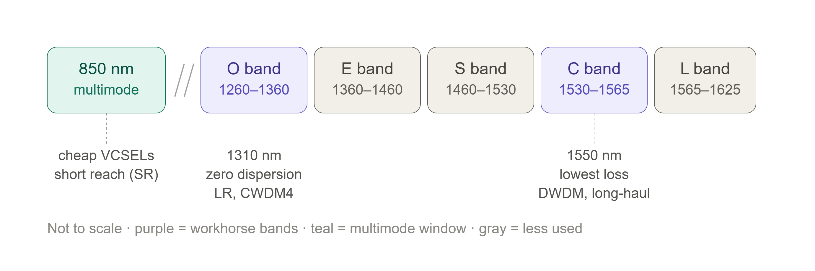
Above you can see the different band groups, their attributes, and their usage. For example:
- O band is known for the near-zero chromatic-dispersion region of standard single-mode fiber. This means very little wavelength-dependent pulse spreading around 1310nm — not that the light exhibits no bending.
- C band is very useful for long-haul, because the light waves in the band showcase very low loss compared to other bands — where loss is how far a light can reach before its brightness decreases.
An example to tie it all together (since it’s worthwhile, and physics is unfortunately complicated):
Assume you have two lasers firing from space — one firing the color red (wavelength at ~650nm) and the other blue (wavelength at ~450nm). When that light passes through the air, it goes through a refractive index that’s very low, so no refraction really occurs to the visible eye. However, that laser then reaches water, and the refractive index of water is higher than that of air — the result is refraction! Both lasers bend, but by different angles: that’s angular dispersion, the prism-style effect shown above. Inside a communications fiber, the chromatic-dispersion problem is instead that different wavelength components travel at slightly different speeds and spread a pulse over time.
Wavelengths & bands, dispersion, refraction, and the refractive index are all very relevant for the upcoming parts in this chapter, and in general are worth knowing.
Connectors
A brief look at the most common optical connectors.
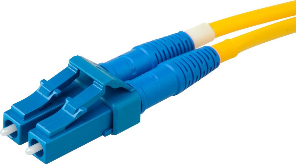
LC — the most widely used optical connector, and today the de-facto standard for transceiver optics. LC is a simplex (single-fiber) connector, but it's almost always deployed as a duplex pair: two LC connectors clipped together, one fiber for TX and one for RX. Its popularity comes from a small form factor and mechanical simplicity — there are no male/female variants. (It does still come in UPC and APC endface polishes, which must be matched to each other.)
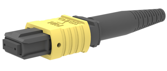
MPO — a multi-fiber connector that's grown popular in high-density environments like AI/HPC datacenters, and the main focus of this section. Where LC-to-LC is simple, MPO introduces real trade-offs.
Importantly, MPO and LC aren’t competitors — they target different use cases and neither replaces the other. And the connector itself isn’t really the point: most of the practical differences come from the cable and transceiver side, covered in the following sections.
The Story of MPO
MPO is an industry-standard connector (defined in IEC 61754-7), originally developed by the Japanese telecom company NTT to improve fiber density and ease of use. (You’ll also see “MTP,” which is US Conec’s tighter-tolerance, trademarked take on the MPO.)
Key differences from LC:
- Fiber count — a single MPO carries many fibers in one ferrule. Common counts are 8, 12, 16, and 24, with high-density variants reaching 32 or even 72.
- Male vs female — MPO comes in pinned (male, two guide pins) and unpinned (female, two guide holes) versions. A pinned connector always mates to an unpinned one, which enforces correct fiber alignment.
- UPC vs APC — MPO endfaces can be flat (PC/UPC) or angled (APC). The angled finish reduces back-reflection (better return loss), which matters most on single-mode links.
So why MPO over LC? Cost and density.
As datacenter speeds climb, so does the cost of the optics — higher baud rates, PAM4 modulation, and precise, expensive lasers. Parallel optics sidesteps some of this: running, say, 8 lanes of 100G over one MPO lets each lane use slower, cheaper components, which can be substantially cheaper than pushing the same aggregate rate down a single fiber pair at a much higher per-lane speed.
Then there’s physical density. One MPO carries 8, 12, or more fibers in the footprint of a single connector, so in a patch panel a single MPO can replace many individual LC terminations — a large density gain for little added cost. In big HPC datacenters, where space, heat, and total equipment count are real constraints, that adds up fast.
Other connectors exist (SC, ST, and more), but LC and MPO are the most prominent today, so they’re the two covered here.
Lastly, it’s worth mentioning that MTP — the trademarked, tighter-tolerance take on the MPO (from US Conec) — has real benefits over a standard MPO, mostly mechanical advantages that improve longevity, ease of use, and alignment tolerances. At the time of writing, though, it’s substantially pricier for a benefit that’s negligible in most deployments.
Transceiver Naming Convention
This segment gives a brief overview of transceiver naming conventions: how to read them, what some of the popular suffixes and prefixes mean, and generally granting the reader an easier way of identifying all the relevant data it can grab from a single read of the transceiver’s details.
The tables here contain only IEEE-accepted fields, and avoid vendor-specific ones as they can be misleading and confusing.
The table beside shows some range-based suffixes, plus a few examples of how to read a transceiver.
Examples:
- QSFP 100G LR4 — Long Reach, 4 optical wavelengths at ~25G each over single-mode fiber
- SFP+ 10G SR — Single lane, Short Reach (indicating multi-mode)
- OSFP 800G SR8 — 8 lanes, Short Reach (indicating MPO Multimode)
| Code | Meaning | Typical fiber / distance* |
|---|---|---|
| SR | Short Reach | Multimode, ~100 m |
| DR | (500 m) | Single-mode, ~500 m |
| FR | Far Reach | Single-mode, ~2 km |
| LR | Long Reach | Single-mode, ~10 km |
| ER | Extended Reach | Single-mode, ~40 km |
| ZR | (long haul) | Single-mode, ~80 km+ |
Wavelength Division Multiplexing
CWDM (Coarse Wavelength Division Multiplexing) and DWDM (Dense Wavelength Division Multiplexing) are two similar technologies that increase bandwidth over a single fiber by multiplexing several wavelengths through the core simultaneously. Each has its own advantages and disadvantages, and this section explains how they work and where each is best used.
It won’t go deep into either one, but aims to provide a baseline for understanding and for applying that understanding to real-world uses.
So far we’ve discussed wavelengths and modulation; WDM is where those two topics come together to deliver real, substantial bandwidth increases, often at lower cost.
CWDM
CWDM operates across a wide wavelength range, 1270–1610nm, spanning from the O-band up to the L-band, with each channel separated by 20nm. That wide spacing is the whole point: it’s loose enough that a laser’s wavelength can drift with temperature without wandering into the neighboring channel, so CWDM can use uncooled lasers (no thermoelectric cooler). That dramatically lowers the cost and power of the optics, which is why CWDM is used primarily in low-cost, short-range applications.
DWDM
DWDM operates in a much narrower range, 1530–1565nm, within the C-band. The reason is amplification: the EDFA (erbium-doped fiber amplifier) only has gain in that narrow window, so confining every channel to the C-band lets a single EDFA boost them all at once as pure light — the foundation of long-haul reach. That’s possible because both the overall range is narrow and the spacing between channels is tight, just 0.8 or 0.4nm. The trade-off is cost: that tight spacing requires cooled, wavelength-locked lasers, and long distances require heavy FEC and DSP to overcome the noise (OSNR decay) and dispersion the signal accumulates along the way.
Per-fiber capacity is the most meaningful way to compare the two. Over a single duplex LC pair, DWDM can theoretically reach tens of Tbit/s — on the order of 32 Tbit/s with modern coherent channels — while CWDM tops out far lower, in the hundreds of Gbit/s, provided you accept the extra cost of the required equipment such as the mux/demux.
Conclusion
This chapter has hopefully helped you grasp the differences between cables, which connector types exist and their advantages and disadvantages, the different types of transceivers, modulations, and multiplexing technologies — whilst also touching on some physics relating to waves and wavelengths, and phenomena such as chromatic dispersion, smearing, and loss: how they occur and how to mitigate them.
The main takeaway from this chapter is that in the complex world of ours, there is no black and white, no “right” or “wrong” solution, no one better cable, no one better technology. Every piece here can, and should, be used correctly in the scenario you’re in to best achieve the goal.